In late 2020 a little-known class of models called diffusion models began causing a stir in the machine-learning world. Researchers figured out how to use these models to generate synthetic images at higher quality than any produced by previous techniques.
Diffusion models are powerful because they generate output through multiple iterations, unlike VAEs or GANs that rely on a single forward pass. This iterative process allows diffusion models to correct mistakes and gradually improve the output, resulting in higher quality synthetic images.
Let's recap over GANs and VAEs first.
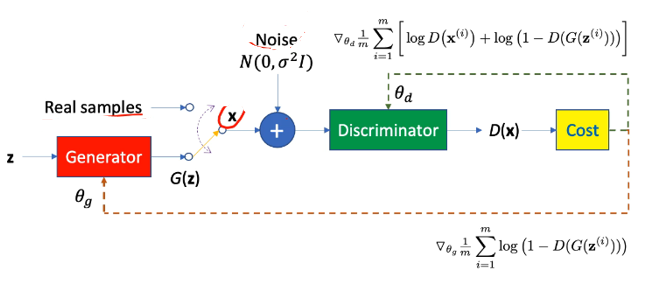
Generative Adversarial Networks (GANs) are a class of machine learning frameworks designed to generate realistic data by pitting two neural networks against each other: the generator and the discriminator. In the image, the process begins with the generator, which takes a random latent vector z (sampled from a prior distribution like \mathcal{N}(0, \sigma^2I) ) and generates synthetic data G(z) that attempts to mimic real samples. The goal of the generator, parameterized by \theta_g , is to produce data indistinguishable from real samples.
The discriminator, parameterized by \theta_d , acts as a classifier that distinguishes between real data and synthetic data. It takes either real samples or generated samples G(z) as input and outputs a probability score D(x) , where D(x) close to 1 indicates real data, and D(x) close to 0 indicates synthetic data. The discriminator's cost function (green pathway) encourages it to correctly classify real data as real and generated data as fake. Simultaneously, the generator's cost function (orange pathway) is designed to "fool" the discriminator into classifying generated samples as real.
The training process involves alternating optimization of the generator and discriminator. The discriminator minimizes a loss function proportional to \log D(x) + \log(1 - D(G(z))) , while the generator minimizes \log(1 - D(G(z))) , encouraging it to produce increasingly realistic data. This adversarial game continues until an equilibrium is reached, where the generator produces data that the discriminator cannot reliably distinguish from real data, effectively creating a realistic data distribution.


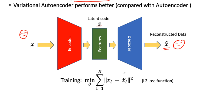
An autoencoder is used for dimensionality reduction and feature extraction. The input data x is passed through the encoder, which compresses it into a lower-dimensional representation, often called the latent code z . This compressed representation captures the essential features of the input data. The decoder then reconstructs the input from z , aiming to produce output \hat{x} , which is as close as possible to the original x .
The autoencoder is trained to minimize the reconstruction loss, typically measured as the squared error ( L2 -norm) between x and \hat{x} . The objective function, \sum_{i=1}^N ||x_i - \hat{x}_i||^2 , ensures that the reconstructed data closely matches the input data.
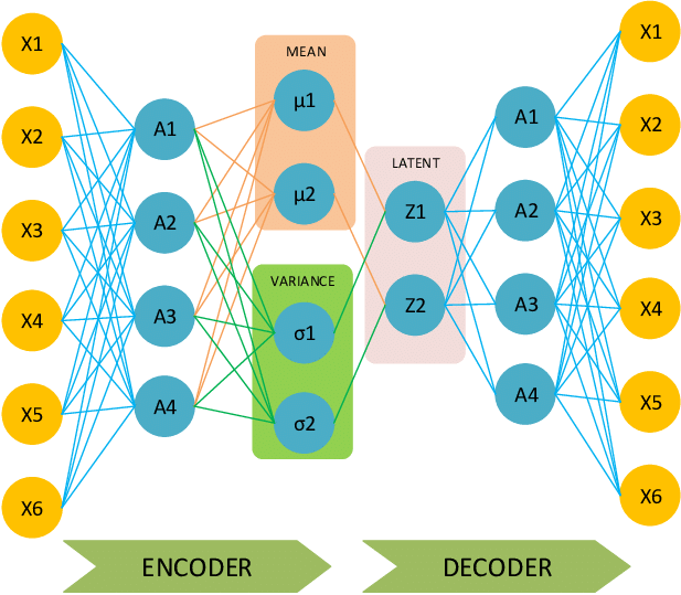
Variational Autoencoders (VAEs) are a probabilistic extension of traditional autoencoders designed for both efficient data reconstruction and generative modeling. The key innovation in VAEs lies in encoding input data x not as a single deterministic point but as a probability distribution in a continuous latent space. Specifically, the encoder outputs two parameters, \mu (mean) and \sigma^2 (variance), which define a Gaussian distribution for the latent representation. This probabilistic framework ensures that the model captures uncertainty in the data and produces a smooth latent space, where small variations in z (samples drawn from this Gaussian distribution) lead to gradual changes in the generated output. The decoder then reconstructs data from the sampled z , ensuring that the generated data resemble the original input while also allowing the model to generate novel data by sampling new z -values.
The choice of a Gaussian distribution for the latent space is deliberate and essential for the VAE's effectiveness. Gaussian distributions are mathematically convenient, as their properties allow for easy computation of the Kullback-Leibler (KL) divergence, which regularizes the latent space during training. The KL divergence ensures that the learned latent space q(z|x) closely approximates a predefined prior distribution p(z) , typically a standard normal distribution \mathcal{N}(0, I) .
The marginal likelihood in a Variational Autoencoder (VAE) is given by the integral:
Where: - p_\theta(x) is the likelihood of the observed data x . - p_\theta(z) is the prior distribution of the latent variable z . - p_\theta(x|z) is the likelihood of observing x given z . - The integral sums (marginalizes) over all possible values of the latent variable z .
The integral \int p_\theta(z)p_\theta(x|z) dz represents the marginal likelihood p_\theta(x) , which quantifies how well the model explains the observed data x across all possible latent variables z .
The integral in the Variational Autoencoder (VAE) framework, \int p_\theta(z)p_\theta(x|z) dz , is intractable primarily because it involves integrating over all possible configurations of the latent variable z . In most real-world applications, the latent space z is high-dimensional, making the computation of this integral computationally prohibitive or impossible to solve analytically.
We integrate over z to calculate the marginal likelihood p_\theta(x) , which represents the probability of the observed data x . This marginal likelihood is crucial because it serves as the model’s measure of how well it explains the data, regardless of the latent variables. In simpler terms, the integration accounts for all possible ways the latent variable z could influence x , weighted by their probabilities under the prior p_\theta(z) . This is key because we don’t observe z directly—it’s a hidden or latent variable that serves to explain the variability and structure in the observed data x .
However, this integration becomes computationally infeasible when the latent space z is high-dimensional. This is because evaluating p_\theta(x|z) (the likelihood of x given z ) for all possible values of z and summing (or integrating) over them involves solving a continuous, complex integral that grows exponentially harder with the dimensionality of z .
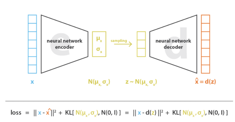
The loss function in a Variational Autoencoder (VAE) combines two components: the reconstruction loss and the Kullback-Leibler (KL) divergence. The reconstruction loss, typically measured as the squared error ||x - \hat{x}||^2 , ensures that the decoded output \hat{x} closely matches the original input x . This term forces the decoder to accurately reconstruct the data from the sampled latent variable z .
The Kullback-Leibler (KL) divergence term in the Variational Autoencoder (VAE) loss serves to regularize the latent space. Let's break it down:
In the VAE, the encoder maps the input x to a probability distribution in the latent space rather than to a single point. This distribution is parameterized by the mean \mu_x and variance \sigma_x^2 , forming a multivariate Gaussian distribution N(\mu_x, \sigma_x) . When the model samples a latent vector z , it is drawn from this Gaussian distribution: z \sim N(\mu_x, \sigma_x) . This sampling introduces variability and ensures the generative capability of the VAE, as z can differ slightly for the same input x .
The KL divergence term \text{KL}(N(\mu_x, \sigma_x) \| N(0, I)) measures the difference between two probability distributions: 1. The posterior distribution N(\mu_x, \sigma_x) , learned by the encoder, which describes how the latent variables are distributed for a given input. 2. The prior distribution N(0, I) , a standard Gaussian with mean 0 and unit variance, which acts as a target distribution for regularization.
The KL divergence penalizes the encoder if the posterior distribution deviates too much from the prior. By minimizing this divergence, the VAE ensures that the latent space remains close to a standard Gaussian, which is critical for generating new samples. This alignment makes the latent space structured, continuous, and well-behaved, allowing the decoder to generate realistic outputs even from latent vectors sampled from the prior N(0, I) .
Breaking it down:
Reconstruction Loss: This ensures the reconstructed output \hat{x} is as close as possible to the input x .
KL Divergence Term: This measures the difference between the approximate posterior q_\phi(z|x) , parameterized by \mu (mean) and \sigma^2 (variance), and the prior p_\theta(z) , typically a standard Gaussian N(0, I) .